Validation and Experimental Design

Biotechnology is one of the most innovative industrial sectors in Germany. Whether in the development of new active ingredients or the production of so-called validation batches for the approval of new drugs, many experiments are conducted daily. Efficient use of time, available raw materials, and personnel is essential for a company’s success. There are differing views on the effort required for validation, which will be addressed here.

The opinion that exactly three validation batches must be produced is widespread. Where does this number come from? The EMEA (1) indicates that for non-standardized processes, especially when sterilization steps or aseptic procedures are applied, at least three consecutive production-scale batches must be manufactured. For other non-standardized processes, one to two production-scale batches may suffice if sufficient data is available from the preceding pilot phase.

In its “Validation Guide” (2), the FDA generally required three batches for validation. And in Annex 15, “Qualification and Validation” (3), of the EU Guidelines to Good Manufacturing Practice, a number of three consecutive batches is described as
“generally acceptable.”

It is always assumed that validation batches are produced under routine conditions. At the same time, however, the texts always refer to the fact that the parameters must be known and that “the number of process runs performed and the corresponding observations are sufficient to determine the normal level of variations and trends and to obtain sufficient data for evaluation.”(3) The FDA guidelines further advise including “worst-case” conditions in the investigations.

At this point, a clear contradiction emerges. On the one hand, variations and trends affecting critical process parameters are to be determined, while on the other hand, 1 to 3 batches are required.

In practice, therefore, the approach is often taken that three batches are produced, but no critical parameters are changed, even if ranges for these were specified in the approval documents. However, the informative value of three investigations is likely to be limited. It is therefore up to the manufacturer to conduct more extensive tests, either beforehand or only after the validation batches, which actually cover the ranges and allow a statement about trends.

In September 2004, the FDA published a recommendation that addresses this problem, among others. Under the term Process Analytical Technologies, a regulatory framework is created to promote the voluntary integration of innovative technologies into the development, production, and quality control of medicines (4). This also addresses the strategy for conducting experiments and recommends the application of Experimental Design (DOE – Design of Experiments). The guideline on validation is therefore currently under revision. A detailed recommendation does not yet exist.

However, as a reaction to the PAT initiative, the term conformance batches was coined in CFR 490.100 (5):

“Before commercial distribution begins, a manufacturer is expected to have accumulated enough data and knowledge about the commercial production process to support post-approval product distribution. Normally, this is achieved after satisfactory product and process development, scale-up studies, equipment and system qualification, and the successful completion of the initial conformance batches. Conformance batches (sometimes referred to as “validation” batches and demonstration batches) are prepared to demonstrate that, under normal conditions and defined ranges of operating parameters, the commercial scale process appears to make acceptable product. Prior to the manufacture of the conformance batches the manufacturer should have identified and controlled all critical sources of variability.”

For pharmaceutical manufacturers who want to produce for the US market, the specific requirement for three conformance batches is thus eliminated. Now, the existing investigations must be used to demonstrate that the critical parameters and all causes of their variability have been identified and controlled. This has brought development and production closer together again, as validation can now only be seen as the concluding part of product development. One of the consequences is that the execution and planning are integrated into an overall concept that also includes a statistically based experimental design.

To understand the validation procedure, the principle of experimental design will be briefly presented. In every process, there are important and less important influencing factors. If one considers, for example, a fermentation process, the following parameters will exert an influence:

• Temperature
• pH value in the culture medium
• Composition of the culture medium
• Inoculum/medium ratio
• Mixing (e.g., stirrer speed)
• Oxygen supply

Depending on whether the influencing factors can be varied or not, they are referred to as control variables or disturbance variables, respectively. The latter must be considered when developing robust processes.

For each influencing factor, a range of validity within permissible limits results. If only certain values within these limits are considered in the experiment, these are called factor levels.

Let’s assume that only temperature and pH value have been identified as critical parameters. How could both factors be set in a validation? To cover the range, we choose the upper and lower range limits. If all possible combinations are now considered, four experiments are obtained.

First, it will be demonstrated how the corresponding plan is constructed. For this purpose, a column is created for each factor in a table. Table 1 first contains as many rows as experiments are necessary.

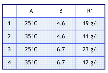
Table 1: Example of a full factorial design

Furthermore, we assume the following values: Temperature (Factor A) in the range of 25°C to 35°C; pH value (Factor B) in the range of 4.6 to 6.7. In the respective row, the factor level combination can now be read. An outcome (R1) for the yield was also entered in the last column. When realizing the experiments, care must be taken to randomize the order. For example, by drawing lots, we get the sequence: 2, 1, 3, 4

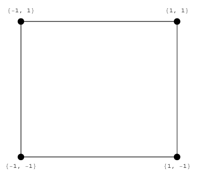
Figure 1: Distribution of experiments as factor level combinations

Figure 1 shows how the points are distributed in the experimental space. Here, the factor levels were generally coded with -1 for the lower and +1 for the upper. It can be seen that two experiments are available for each, which were carried out at a low and a high level of the factor under consideration. If one wants to quantify the effect, the mean of the measured results is formed at the lower and upper factor levels. Subsequently, the difference between the means is formed. If the differences for the individual effects are compared, a sequence is obtained. The larger the difference, the greater the influence of the associated factor.

Diff A= (11+12)/2-(19+23)/2=-9
Diff B= (23+12)/2-(19+11)/2= 3

It follows that the influence of factor A is greater than that of factor B. Furthermore, it can be seen that A worsens the yield, while B increases the yield.

Table 2 shows the general coding of the effects and simultaneously represents a kind of calculation scheme. The procedure is to multiply the coded values from a column by the result column, then sum the results. The sums must be divided by the number of values used for calculating the mean. In MS Excel, this calculation can be quickly determined using the “SUMPRODUCT” function.

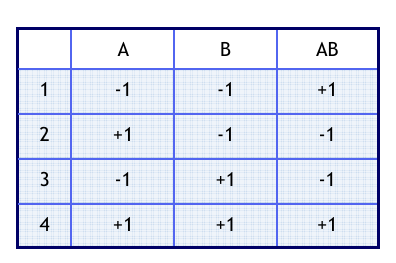
Table 2: Coded factor levels

The table shows another column. Column AB results from multiplying columns A and B. With the column vector AB, the interactions between the factors can now be calculated using the same scheme. Interactions are always important when the change of one factor also has an influence on another factor. This is exactly what is shown in Figure 2.

Our example only considered two factors, for which we set up a full factorial design. If more factors are to be considered, the number of experiments grows exponentially. The number of experiments can be reduced by setting up so-called fractional factorial designs.

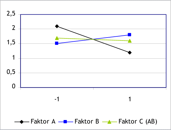
Figure 2: Mean comparison for factors A, B, and C

In this case, interactions are used. If there is no interaction between A and B, it can be “confounded” with another factor C. From Table 2, one can read in column AB which level must be set for factor C. In this way, 3 factors can be investigated with a factorial design for two factors. The number of experiments is as follows:

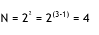
This type of reduction is very efficient, as neglecting an interaction halves the total effort. However, it is important to determine the factor levels exactly according to the pattern in Table 2, as this is the only way to achieve an even distribution in the experimental space. The following example illustrates the reduction of experiments. We start with a full design with 3 factors, so 8 experiments are necessary. The factor levels in their coded form can be represented by points of a cube.

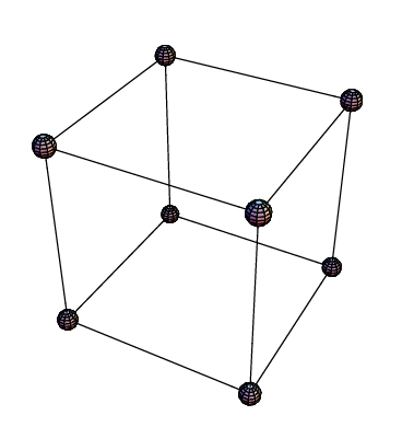
Figure 3: Factor level combinations for 3 factors

Here too, the effects are determined by forming means of all experiments that were carried out, for example, for factor A at level -1 and +1. This can be imagined as comparing the results of two opposite cube faces. If a reduced factorial design is to be set up, the experiments must remain evenly distributed in the experimental space.

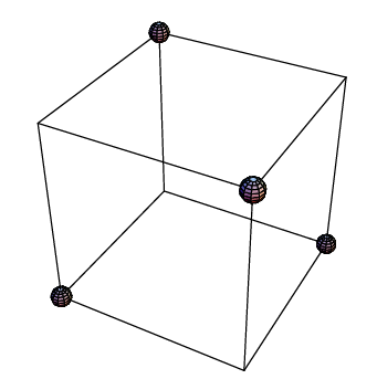
Figure 4: After reduction, each cube face has the same number of experiments

This ensures that the number of experiments per cube face remains the same on all sides even after reduction. By projecting the cube corners, the representation in Figure 1 is obtained. This reduction is also possible in experimental designs with more than three factors. Several interactions can even be confounded with new factors. For example, a 2(6-3) design requiring only 8 experiments can be constructed with the six factors mentioned at the beginning.

The magnitude of the calculated effects is a measure of the magnitude of the factors’ influence. Statistical calculations are often supported by so-called significance tests. The validity of a statement is limited by assuming a certain probability that the statement is false. Error probabilities of 5, 1, or 0.1 percent are often used. With these, the 95, 99, and 99.9 percent confidence intervals are calculated. For the calculation of confidence intervals, for example, the t-test is used. However, the t-test is only applicable if so-called degrees of freedom exist. Behind the calculation of the effects lies a mathematical model that estimates parameters. If the model is used for a 2³ design, 8 parameters are estimated, i.e., exactly as many as experiments are performed. This leaves no degrees of freedom.

Degrees of freedom are only gained by repeating experiments. The complete repetition of an experimental design is widespread. However, this doubles the effort. If one knows one’s experimental setup very well and can estimate that the variance between repetitions is the same for all factor level combinations, the effort can be reduced. In this case, a single experiment is repeated twice. Now the variance can be estimated, and with the two degrees of freedom obtained, the t-test can be performed and a confidence interval for the effects can be given. If the effects lie outside these calculated confidence intervals for 95, 99, or 99.9%, it can be stated that the effects are significant at the respective level. If the effects remain within the confidence intervals, the effects are indistinguishable from random errors.

Conformance batches are to be produced for a freeze-drying process. Two products are manufactured and filled in 5 different dosages from 2 to 20 ml. The effort is reduced by only considering the filling of the largest and smallest quantities here. Freeze-drying is carried out with a standard program that was adopted from a smaller system. For the duration of the main drying, a possible reduction in time from 24 h to 20 h is assumed due to scale-up. The size of the batches varies as needed between 10,000 and 20,000 bottles. With these influencing factors, a fractional factorial design with 2(4-1)=8 experiments is defined. Now, further experiments are necessary to determine the experimental variance. For this, a factor level combination is chosen from which, based on process knowledge, the greatest variance in the investigated results is expected. This factor level combination is realized at least twice in addition to the experimental design. The experimental design now contains 10 experiments. It is important that all experiments are randomized, including the additional experiments.

The target variables chosen are water content, active ingredient content, appearance, etc. After execution, the effects and interactions are calculated. Using t-statistics, the confidence limits for the effects are determined. Now it can be assessed whether effects occur. In the case of validation, the effects and interactions should all lie within the confidence limits, i.e., have no significant influence. This would demonstrate a robust process.