Densest Packing of Cylindrical Containers on Flat Surfaces

Pharmaceuticals are often filled and stored in cylindrical containers with a circular base. In this process, the bottles are arranged as closely as possible (Fig. 1).

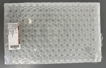
Fig. 1: 6R vials in delivery packaging

Such arrangements lead, among other things, to the question of the maximum number of bottles on a given area1, as well as the total mass of the bottles. If these are placed next to each other in the x and y directions, a pattern with square fields is obtained, as shown in Figure 2. Each bottle touches its two neighbors in each direction.

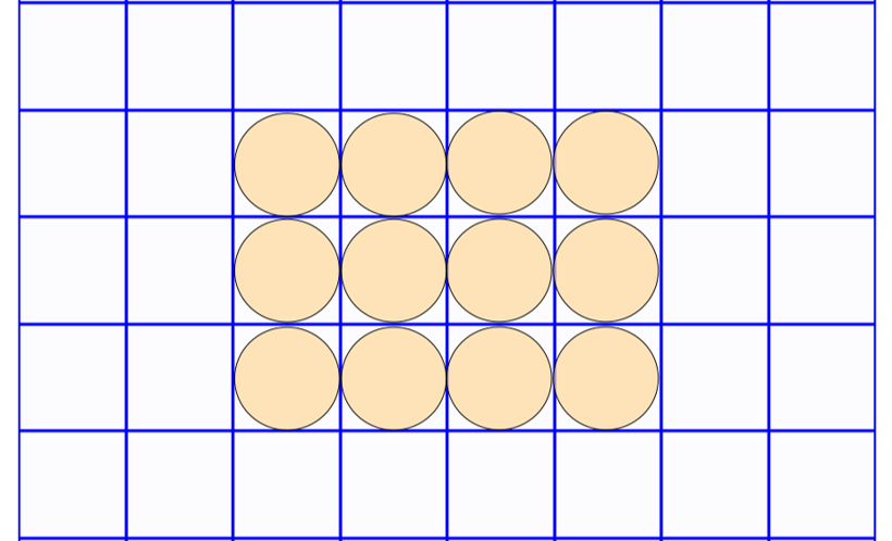
Fig. 2: Tessellation with quadrilaterals

If the bottles are consistently arranged with a row offset, a hexagonal pattern is created (Fig. 3) in which one bottle touches six others. This pattern represents the most efficient use of space, which the mathematician Joseph Louis Lagrange proved in 1773, calculating the value of the packing density as (pi/sqrt{12}approx 0.90690). [1].

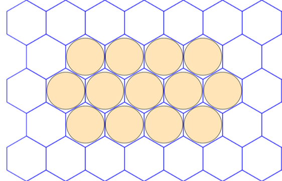
Fig. 3: Tessellation with hexagons

Hexagonal arrangements are frequently encountered in nature, e.g., honeycombs and soap bubbles. The honeycomb structure (Fig. 4) allows bees to obtain the maximum storage space for pollen, honey, and their larvae with a minimum use of wax and energy.

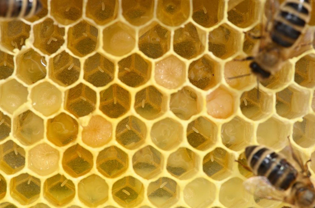
Fig. 4: Tessellation with hexagons

In 1873, the Belgian physicist Joseph Antoine Ferdinand Plateau (*1801; †1883) published his findings from the observation of soap films. One of his findings was that soap films always meet in threes at an angle of 120° [3]. The interior angles in an equilateral

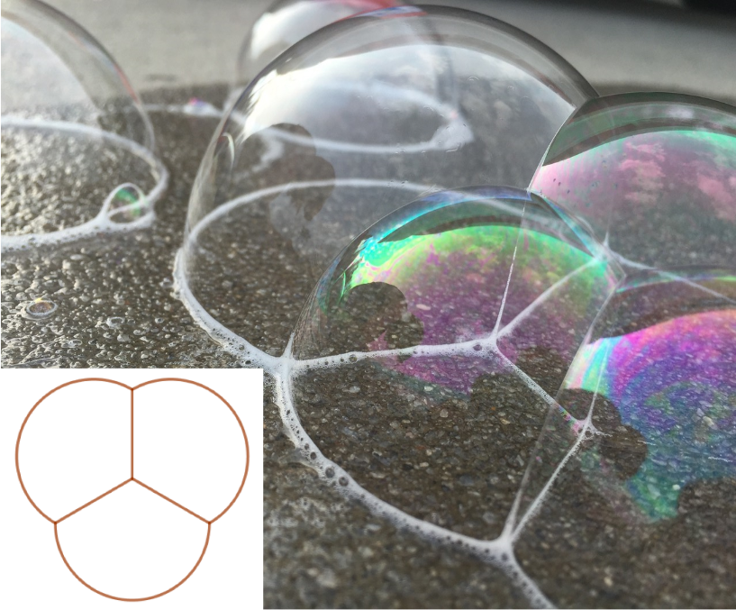
Fig. 5: Angle between edges of soap bubbles

hexagon are also 120°. Given this geometric parallel, the preference for a hexagonal arrangement in technical processes becomes understandable.

(^1) The gapless and overlap-free arrangement of uniform sub-areas is referred to as tessellation.

During production, bottles with the same circular diameter are always used for a batch. When these are lined up as closely as possible, the densest possible arrangement is created. In this case, each circle (except at the edges of the pack) touches six surrounding circles.

If you start placing bottles next to each other at a straight edge, a gap often remains at the end of the edge. The next row

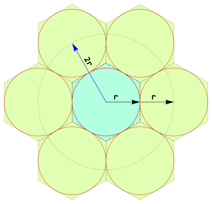
Fig 6: Hexagon with adjacent hexagons

is arranged with an offset; the row after that starts again at the beginning of the edge, offset accordingly to the previous row. To determine the offset, the centers of three touching circles are connected. This results in an equilateral triangle with an interior angle of 60° in each corner. The perpendicular a from the apex of this triangle to the opposite side bisects it and thus forms a right-angled triangle (Figure 7).

$$a^2 + b^2 = c^2$$
$$a^2 = (2r)^2 – r^2$$
$$a = sqrt{3}r$$

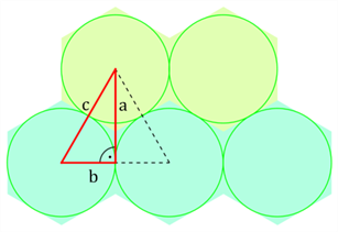
Fig. 7: Determination of the offset

The length of the segment a is obtained using the Pythagorean theorem. The offset to the next row corresponds to the radius multiplied by (sqrt{3} approx 1.73).

A square unit area A with an edge length of k is to be defined. At the edge in the x-direction, the circles with diameter d are lined up next to each other until the first row is full. The edge length is divided by the diameter and the remainder (S_x) is determined (Fig. 8, Eq. 1). If this is subtracted from the edge length (k_x) and divided by the diameter (d), the number (n_x) of circles in this row is obtained.

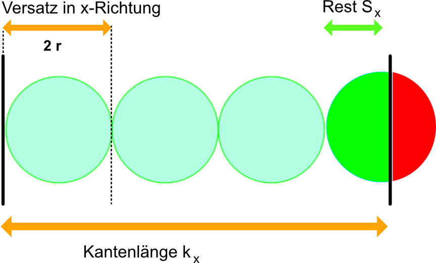
Fig. 8: Determination of the number in the first row (x-direction)

$$S_x = k_x mod d quad(1)$$
$$n_x = rac{k_x – S_x}{d} quad(2)$$

With the 10R format (d = 24 mm), the number in the first row is obtained as follows.

$$16 = 1000 mod 24$$
$$41 = rac{1000 – 16}{24}$$

In practical use, rounding down to a whole number (n_x) is easier after dividing the available length by the diameter of the vial.

$$left[rac{k_x}{d} ight] = n_x quad(3)$$
$$rac{1000}{24} = 41.7 ightarrow 41$$

Similarly, the number of rows in the y-direction is determined using the row offset (rsqrt{3}).

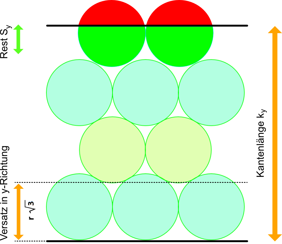
Fig. 9: Determination of the number of rows in the y-direction

$$
egin{aligned}
S_y &= k_y mod r sqrt{3} \
n_y &= rac{k_y -S_y}{rsqrt{3}}
end{aligned} quad(4)
$$

$$2.34 = 1000 mod 12sqrt{3}$$
$$48 = rac{1000 – 2.34}{12sqrt3}$$
$$100$$

As a simple approximation, the edge length can be divided by the row spacing. The value is again rounded down to an integer.

$$left[rac{k}{rsqrt{3}} ight] = n_y quad(5)$$
$$rac{1000}{12sqrt{3}}= 48.1 ightarrow 48$$

To determine the total number N of bottles, the specific dimensions of the footprint must be taken into account. At the edges, there are four possibilities for filling the gaps. For this purpose, a distinction is made between rows with odd (index (u)) and even ordinal numbers (index (g)). While the rows in cases a and b contain the same number of bottles (n_u = n_g), this is not the case in cases c and d: (n_u = n_g − 1). The situation is similar

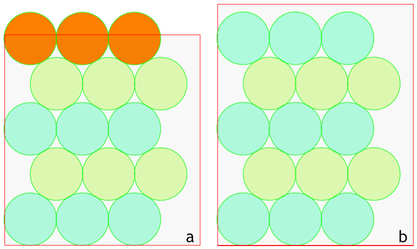
Fig. 10: Rows with the same number n of bottles ($n_g = n_u$)

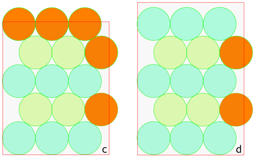
Fig. 11: Rows with an unequal number of bottles (n_g = n_u – 1)

with the number m of rows. Cases a and c have an even number of rows, while cases b and d have an odd number of rows. This must be taken into account when determining the total quantity of vials on the area. The number of rows with an even ordinal number (m_g) must be multiplied by the number of bottles (n_g) contained therein. The same procedure is followed for the rows with odd ordinal numbers. The total number N results from the addition of the vials in odd and even rows.

$$N = m_u cdot n_u + m_g cdot n_g quad(6)$$

In the examples, only very few bottles were shown to make the principle understandable. The gaps are not optimally utilized in these cases. As the size of the area increases, the ratio of the densest packing to gaps at the edges becomes larger and approaches the maximum value of 90.7%.

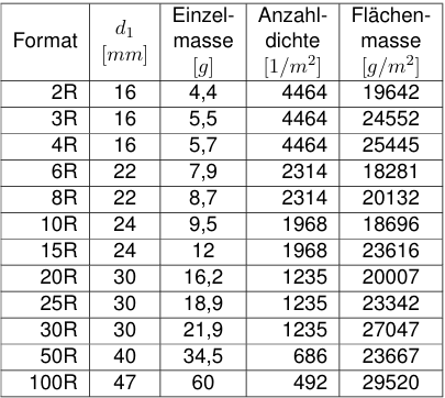
The mass of the bottles on the footprint results from multiplying the number according to Equation 6 by the individual mass per container. Injection containers on a square area with an edge length of one meter shall serve as an example. Table 2.5 provides an overview of the formats defined in ISO 8362-1² [2]. The highest packing density of 89.7% is achieved with the 2R, 3R, and 4R vials, which are characterized by their small diameter and consequently have the smallest gaps. Conversely, the 100R vials only reach a packing density of 85.3%. This shows that as the footprint decreases, the packing density drops and the differences between the formats become more pronounced.

Tab. 1: Number density and mass per unit area per (m^2) for injection containers according to ISO 8362-1

(^2) ISO 8362-1 designates the outer diameter of the injection containers as (d_1).

The legally required verification of the success of sterilization and depyrogenation requires precise and complex measurement of the temperature distribution within the bottle arrangement. Furthermore, the reliable elimination of spores as well as the destruction of endotoxins must be demonstrably reproducible. Given these demanding requirements, it appears appropriate to limit the scope of investigation by focusing on a selection of specific formats. Let us take the example of a manufacturer who wishes to fill their products into the following formats: 2R, 6R, 10R, 20R, and 30R. Considering the glass mass per area according to the table above, the following situation arises. The 2R format is a light representative of the 16 mm diameter in terms of mass. The 6R format is a representative for 22 mm and has the lowest mass per unit area of all formats. The 10R format represents a diameter of 24 mm. The 20R and 30R formats, on the other hand, have a diameter of 30 mm. The 30R format has the largest mass per unit area of 27 kg per m². This format must therefore be taken into account in any case. Whether further formats are included depends on the assessment of the heat transfer.

First, cells are defined for entering the width (in cell B1) and the depth (in cell B2) of the area, and variable names are assigned to the cells. The corresponding value can be entered into these cells. Subsequently, the actual calculation is performed, which is set up in columns A to N. The corresponding column headings are placed in row 3 and the formulas in rows 4 to 15. As an example, the content of row 4 is explained, based on a width of 450 mm and a depth of 620 mm. For comparison, the alternative calculation by rounding is listed in columns N to Q.

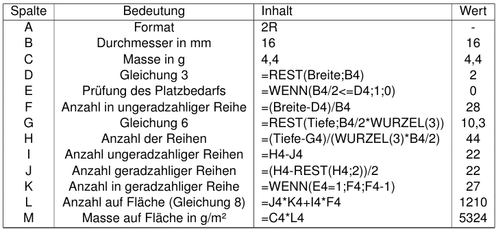
Tab. 2: Calculation using the Remainder function, example for width 450 mm and depth 620 mm

Tab. 3: Calculation by means of rounding, example for width 450 mm and depth 620 mm