Particle Transport Through Leaky Facades

The effect of wind on structures has been extensively studied in recent decades, see [1]. During a severe storm with wind speeds of 100-150 km/h, a stagnation pressure of 500-1,000 Pa is generated on the windward side of a building. These forces must, of course, be taken into account in the structural analysis of the building and in the design of its components (e.g., facade elements).

However, wind load also leads to infiltration, i.e., the penetration of outside air through building joints and thus to natural ventilation of the building. When designing heating and air conditioning systems, infiltration is considered by calculating the ventilation heat demand. In buildings where pharmaceutical products are manufactured, infiltration additionally causes contamination, because the aerosol particles dispersed in the incoming outside air are carried into the building. To protect cleanrooms against this contamination by infiltration, a room-within-a-room construction is often chosen, meaning, for example, that the cleanrooms are preceded by surrounding “black” corridors, which form a protective barrier against direct particle ingress. Due to the scarcity of building space, cleanroom areas are increasingly being extended and utilized right up to the exterior wall. This makes the exterior wall a cleanroom wall with particularly high building physics requirements: freedom of expansion due to thermal load changes (ΔT = 60-80 K), high joint tightness even under extreme wind load, high diffusion tightness, and good thermal insulation to prevent condensation and mold growth on the interior wall surface.

This paper will specifically examine particle transport through facade joints and its influence on cleanliness. The question is: how tight must a facade be to reliably maintain a cleanliness class C (in operation) according to the EU GMP Guide, Annex 1 [15] in the cleanroom in the long term?

We assumed a room with an area of L_R B_R = 10 m 10 m = 100 m² and a height of H_R = 3 m as a model. The model room volume is thus 300 m³. With a supply air-room air change rate of β=20 1/h, the supply air volume flow rate is ˙ V_zu = 6,000 m³/h. A wall surface of 10 m X 3 m = 30 m² is to be an exterior wall, through which, at a wind load of 500 Pa, the infiltration flow rate ˙ V_INF = μV_ZU can flow, where = migration coefficient.

The HVAC system underlying the model equation is shown in Fig. (1). It consists of an outdoor air pre-treatment unit and a recirculation unit. Since we are exclusively considering particle transport, only the filter stages are shown in the system diagram. It is assumed that the components present in the units (especially the fans and humidifiers) are not particle producers themselves. The 8 filter stages shown in the diagram (3 in the outdoor air unit, 3 in the recirculation unit, and 1 terminal filter each in the supply air and exhaust air) are merely intended to represent position and configuration variants. For the development of calculation equation (22), it was necessary to include all variants (placeholders or dummy positions). For the computational simulation of a

real system, all unneeded filter variants are eliminated by setting the corresponding penetration P_j to one. A filter with a penetration P = 1 allows all particles to pass through, meaning it is computationally absent. The following sections (2 to 6) explain the fundamentals required for establishing the calculation equation.

Number concentration or number density and particle size distribution (PSD) are fundamental quantities in aerosol physics for describing the properties of particle collectives. It is therefore very surprising that these basic concepts are not adequately defined in the literature, see e.g. [2, 3, 4]. According to Ziemer [5], the following terms must be distinguished:

1. local, cumulative number concentration

2. local, fractional number concentration

3. particle size distribution (PSD)

The quantities mean: δN = number of all particles of size D > 0, dispersed in δV at time t and location r. The dispersion medium is considered a continuum, which as such has no discrete structure. Then all particles with the property D > 0 are in principle countable. δV = elementary volume element around point P(r) from the control volume (CV) V, small enough to justify the application of infinitesimal calculus, but still large enough to contain a sufficient number of particles δN to perform particle size statistics according to Eq. (3). d(δN) = monodisperse fraction of δN, i.e., number of particles in the size interval [D; D + dD], dispersed in δV at time t and location r. f(Dr t) = frequency density of the PSD by quantity type “number”.

Eq. (2) is rearranged for d(δN) and then integrated over the CV:

When integrating the left side of Eq. (4), we used the commutative property of the operators “d” and “δ”. The substantial derivative is now formed from Eq. (4):

where dN/dt = N˙ = cumulative particle flux for particles with D > 0 and d(dN/dt) = dN˙ = fractional particle flux or fractional particle flux for particles from the monodisperse particle size range [D; D + dD]. The fractional particle flux in Eq. (5) is further split into source and sink fluxes: dN˙ = dN˙_q − dN˙_s . Thus, the conservation law of particle number is:

The left side of Eq. (6) describes the purely convective transport of particles to/from the CV. The right side of Eq. (6) represents generalized source and sink fluxes, i.e.:

• a) Inflow / outflow of particles of the monodisperse fraction [D; D + dD] across the boundaries of the CV due to non-convective phenomena (inertia, sedimentation, diffusion due to Brownian motion, etc.)
• b) Increase / decrease in the number of particles of a considered fraction [D; D + dD] in the CV due to coagulation, condensation, or evaporation
• c) Particle sources and sinks in the CV, which may exist as discrete generators or adsorbers, or may be quasi-continuously distributed in the CV.

The substantial derivative according to Euler is:

where v = vector of the velocity of the dispersion medium

We consider the special case of a stationary flow tube. Due to stationarity, ∂(dC)∂ (t) = 0. The remaining part of the volume integral is converted into a surface integral using Gauss’s integral theorem:

where n = the outward-pointing unit vector of the surface normal. For the simple flow tube, the surface integral can be calculated with the following assumptions:

• a) cross-sections A1 and A2 are perpendicular to the axis of the flow tube, i.e., vectors v1 and n₁ and v₂ and n₂ run parallel to each other, so that v₁ · n₁ = −v₁ and v₂ · n₂ = +v₂. On the mantle of the flow tube, v_O · n_O = 0
• b) The fractional number concentration, PSD, and velocity are constant on cross-sections A₁ and A₂.

This gives us

The quantities vj A_j = V˙ _j are known to represent volume flow rates. For stationary flow in a general flow tube with many inlet and outlet surfaces, the following applies:

The subsequent calculation equation is based on the balance of fractional particle fluxes, which is written in the following form using Eq. (3):

Particle fluxes through channels and rooms can be approximately treated one-dimensionally using the aforementioned streamline theory if cross-sectionally averaged values are used for velocity, number concentration, and PSD.

The atmospheric aerosol influences cleanroom purity in two ways:

• a) Outside air is drawn in by the HVAC system, and the aerosol contained therein enters the cleanroom, albeit attenuated in number concentration and PSD by the various filter stages,
• b) through small gaps in the exterior facade, outside air penetrates unfiltered into the cleanroom under appropriate wind load.

To computationally estimate these influences, it is necessary to know the number concentration and PSD of the atmospheric aerosol (preferably also the microorganism content). The first systematic measurements were carried out by C. Junge in the spring of 1951 at the Meteorological Institute in Frankfurt am Main. Junge [6] measured the number concentration and PSD of 25 continental aerosols and found a remarkable constancy of the distribution in the particle size range D = 0.2 … 10 µm:

The logarithmic fractional density could be represented by a power law distribution, with the exponent ν ≅ 3. This distribution became known as the Junge distribution. Today, the atmospheric aerosol is usually described by a tri-modal LNVT corresponding to the 3 components (modes) that have been identified:

• 1. NM = Nucleation Mode, consisting of ultrafine particles of size D 0.1 µm with high number density
• 2. AM = Accumulation Mode, consisting of submicron particles of size D = 0.1 … 1 µm with medium number density
• 3. CM = Coarse Mode, consisting of fine and coarse dust particles of size D > 1 µm with low number density.

The fractional number concentration of the atmospheric aerosol is thus described as follows:

with F_AU (D) = fractional density in 1/m⁴ or 1/(cm³ µm) as shorthand for the formula in square brackets.

The LNVT components are as follows

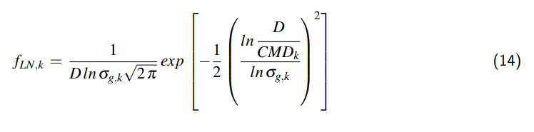
Each component k is described by 3 parameters: C_k = cumulative number concentration, CMD_k = median diameter, and σ_g,k = geometric standard deviation.

We decomposed the urban aerosol measured by Junge in Frankfurt a. M. into a tri-modal LNVT and summarized the 9 parameters in Table (1).

Contamination is predominantly caused by humans and their activities. We therefore focused on particle emission by people working in the cleanroom and neglected particle generation by production machines or processes. This is also because no reliable data is available on these.

Minamino [7] conducted a series of excellent measurements on human particle emission depending on activity level and cleanroom garment type. We re-evaluated his values and found that they can be represented by a bimodal LNVT in the size range D = 0.3 … 15 µm, for both low and high activity.

Low activity is defined by slight arm movements while sitting, high activity by
walking, standing up/sitting down, and exercise. The cleanroom garments consisted of a coverall, arm
protectors, overshoes, and a hood. The coverall was made of lint-free 100% polyester and was electrostatically dissipative due to woven carbon fibers spaced 5 mm apart.
Fig. (5) shows the cumulative particle flux per person as a function of particle size:

with the two activity levels as parameters. The 2 x 6 parameters (N˙_j ,CMD_j ,σg _j) are summarized in Table (3). From the room-side particle flux balance, the fractional particle flux dN˙_q produced by humans is converted into a fractional number concentration dC_q:

with n* = occupancy density (number of persons per area), β = supply air-room air change rate, H_R = room height, and F_q(D) = fractional density of particle sources in the room.

In cleanroom technology, two types of air filters are used: standard air filters for pre-filtration, whose filtration performance is classified according to DIN EN 779 [13], and HEPA filters according to DIN EN 1822-1 [14]. Both standards implicitly assume that the filter media consist of fibers.

Based on the current state of our knowledge in aerosol physics, especially filter theory, and available aerosol measurement technology, the two filter standards show significant differences in testing methodology. The classification of HEPA filters according to DIN EN 1822-1 is based on fractional penetration by “number” at the MPPS = Most Penetrating Particle Size. For the classification of pre-filters according to DIN EN 779, two filter classes must first be distinguished: coarse dust filters (G1 – G4) and fine dust filters (F5 – F9). Only fine dust filters are relevant for cleanroom technology. These are challenged with DEHS according to DIN EN 779. The collection efficiency is determined for 0.4 µm.

For modeling, we made a simplifying distinction between HEPA filters with polydisperse fibers

and pre-filters with monodisperse fibers

where α = mean fiber volume fraction (packing density), L_F = thickness of the filter medium, D_f = fiber diameter, D*_f = effective fiber diameter, { D_f } = mean fiber diameter, { D²_f } = mean fiber diameter squared, ε1 and ε2 = correction factors for adaptation to experimental values,

η = single fiber collection efficiency. The structural data used are summarized in Table (2). The single fiber collection efficiency η was calculated for the case of polydisperse micro-glass fibers of HEPA filters according to the theory of Fuchs-Stechkina-Kirsch [8,9]. For the case of monodisperse pre-filters, we used the simplified theory according to Lee [10] in combination with Rubow’s slip correction [11].

The derivation of the calculation equation can only be outlined here; for more details, see the paper by Ziemer and Schenderlein [5]. First, a room-side balance of fractional particle fluxes is established:

On the left side is already the desired quantity dC_R, on the right side the still unknown quantity dC_ZU , which is determined from a system-side balance:

Now, Eq. (20) is substituted into Eq. (19) and rearranged for the desired quantity dC_R:

To enable a comparison with the cleanliness classes according to ISO 14644-1 or the EU GMP Guide, Annex 1, which are known to be cumulative PSDs, Eq. (21) must be integrated:

The quantities mean: α* = α/(1−λ) = the outdoor air fraction reduced by the leakage air fraction, with α = V˙_AU /V˙ _ZU = outdoor air fraction and λ = V˙ _LE/V˙ _ZU = leakage air fraction, µ = V˙ _INF/V˙ _ZU = migration coefficient, i.e., the outdoor air fraction that penetrates the cleanroom through the facade joints due to wind load (infiltration), ε = ventilation effectiveness, P₁₋₇ = product of the fractional penetrations of filters (1) to (7) and P₄₋₈ = likewise for filters (4) to (8). The penetrations are calculated according to the procedures described in Section (5).

Fig. (6) shows typical PSDs that would occur in the cleanroom under operational conditions (in operation) and under the influence of varying degrees of outdoor air infiltration. The chosen filter configuration consisted of a pre-filter P₄ = F7 and a post-filter P₆ = F9 in the recirculation unit (P₁ = P₂ = P₃ = P₅ = 1 set). Furthermore, a terminal HEPA filter P₇ = H 14 was used, and a room-side exhaust air filter was omitted (P₈ = 1). In the lower curve (µ = 0%, ideally tight facade), the contamination by people present in the cleanroom can be seen in the right part. It is low due to the low occupancy density (1 person/50 m² ), approximately C = 2,500 1/m³ or 70 1/ft³ for D > 0.4 µm.

Below 0.4 µm, human contamination is completely masked by outdoor air particles that penetrate all the aforementioned filter stages. Between D = 0.4 … 0.15 µm, there is a steep increase (approx. 40-fold) in number concentration up to approx. 1 × 10⁴ m³ or 285 1/ft³ . Although this particle size is outside the usual consideration limits in pharmacy, these particles still represent a certain chemical contamination (e.g., ultrafine soot particles). As soon as a certain facade leakage occurs, the aerosol content in the cleanroom increases. At µ = 0.5%, the limit curve for cleanliness class B is already exceeded. If one calculates the specific leakage air rate γ = V˙ INF/AW, one obtains:

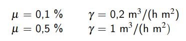
If one wants to reliably maintain cleanliness class C (in operation) according to the EU GMP Guide, Annex 1 [15] in the long term, it is recommended

to maintain the specific facade leakage. The few experimental determinations on facades available so far show that this value can also be maintained.

δ μ ≅